Unit 5: The Mean Value Theorem and applications
There is a common theme in many of the proofs and applications in this Unit: when you use a Theorem, verify the hypotheses first. Students need many reminders of this.
I have not included any activity that works with Video 5.8 (Proof of the MVT). In the past I have tried various things, but none worked well for a class activity. The practice problems contain an exercise to come up with and prove Cauchy’s MVT that works very nicely as a practice problem, but not as a class activity.
I have included various activities to introduce students to the art of coming up with new theorems. It fits well with what they learned in the videos. The activities are nice when they work out, but beware: they look simple, but they are hard, and they take longer than you may expect.
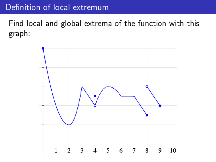
Definition of local extremum
Definition of local extremum
Related Videos
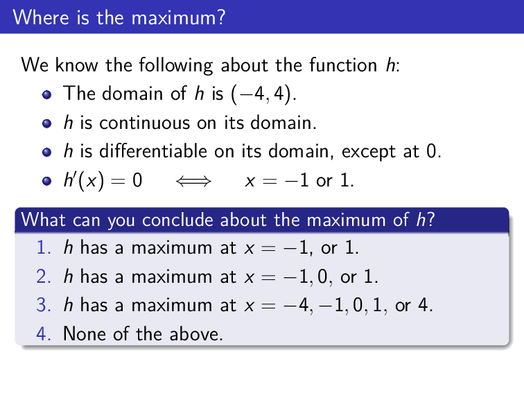
Where is the maximum?
Where is the maximum?
-
The correct answer is that we can only conclude that either has no maximum, or the maximum occurs at , , or .
-
Students favourite algorithm to find extrema is “Find the points with derivative 0. One of them is the maximum”. They forget points where the derivative does not exist, endpoints, and the option of not having a maximum. I blame their high-school teachers.
It is really hard to get them out of the habit. For example, when asked to find the maximum of a function, they search for points where the derivative is 0, and if there is only one, it must be the maximum.
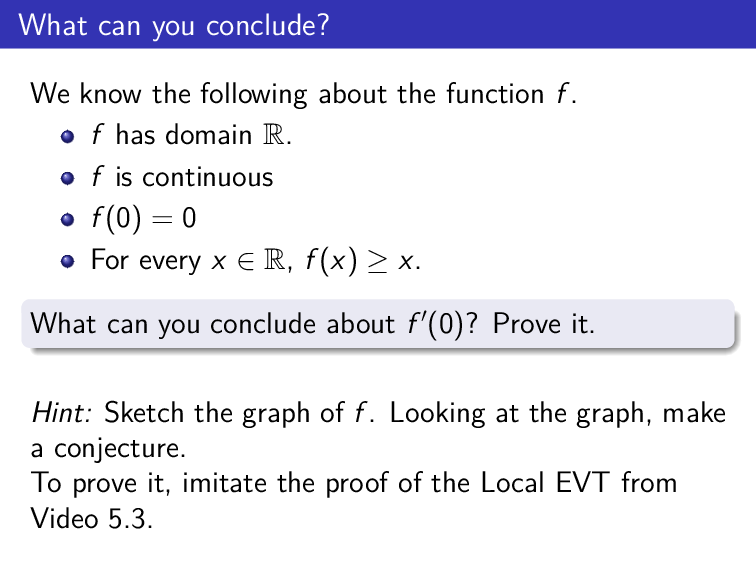
What can you conclude?
What can you conclude?
-
This activity is an attempt to make students think about the proof in Video 5.3. The best way to see if a student understands a proof is to ask them to use the same ideas in a new case. It is not that these proofs are particularly important: we are just practicing proofs in general.
-
The conclusion I am looking for is or DNE. The proof I am looking for is that
-
This activity is pointless if students have not watched the corresponding video. Even then, it is hard. It will take longer than you may think.
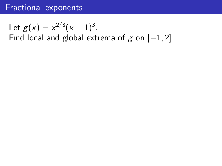
Fractional exponents
Fractional exponents
-
Students know that “to find the extrema of a function” (they do not make distinction between local and global) “find the points where the derivative is 0”. Sadly they often stop at that. The issues:
-
They may forget that points where the function is not differentiable are also critical points.
-
They may forget the end points.
-
More importantly: before we jump into looking at critical points and endpoints, we need to justify the function has extrema (in this case, we invoke the EVT). Otherwise, we are only saying that “if the function has extrema, they must be at one of these points...” It is very difficult to convince students of this last point. If you explain it, they will understand it, but when we ask a question on a test more than half of them will ignore it.
-
-
Students (mostly) take the derivative correctly, but to find the critical points it helps to first “simplify” the derivative and factor it nicely. They have trouble with this.
Trig extrema
Trig extrema
-
The domain is so we cannot invoke EVT. However, the function is periodic. Half of the students will ignore this. The other half will realize it is periodic so we can restrict our domain to . However, they may or may not be comfortable explaining why this is.
-
. This is not a “nice” angle, but it is still possible to find the values of at those points. Students will be uncomfortable with this. Among those who don’t freeze and just wait for you to do it, they may still miss that there are two values of when .
How many zeroes?
How many zeroes?
- This is a simple application, very similar to the one on Video 5.6. Any student who has watched the video should be able to do it.
Zeroes of the derivative
Zeroes of the derivative
-
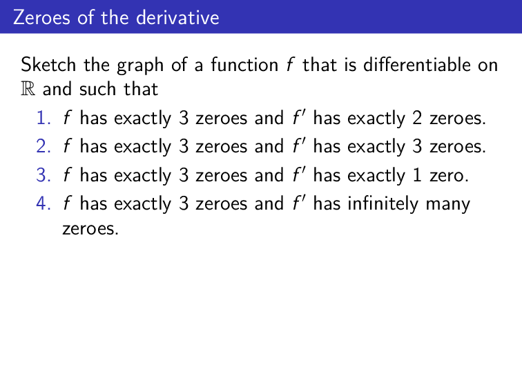
Option 3 is impossible (as explained in Video 5.6). The others are possible, but we still need to sketch an example.
-
In my experience, students don’t have trouble with this question.
-
I often use this as a warm up. I post the question, split the board space in 4, and I walk among them while they work. When I see an example that I like, I give a piece of chalk to the student and ask them to come to the board and draw it.
Zeroes of a polynomial
Zeroes of a polynomial
- Video 5.6 states that the number of zeroes of a function is at least 1 + the number of zeroes of . So that is basically it. This proof is trivial... for us. For students this proof is weird. They are used to the induction step being to manipulate one equation to get another equation. This is different. In a proof like this, they are very uncertain of whether they have “written enough” or even what they are “supposed” to write.
An extension of Rolle’s Theorem
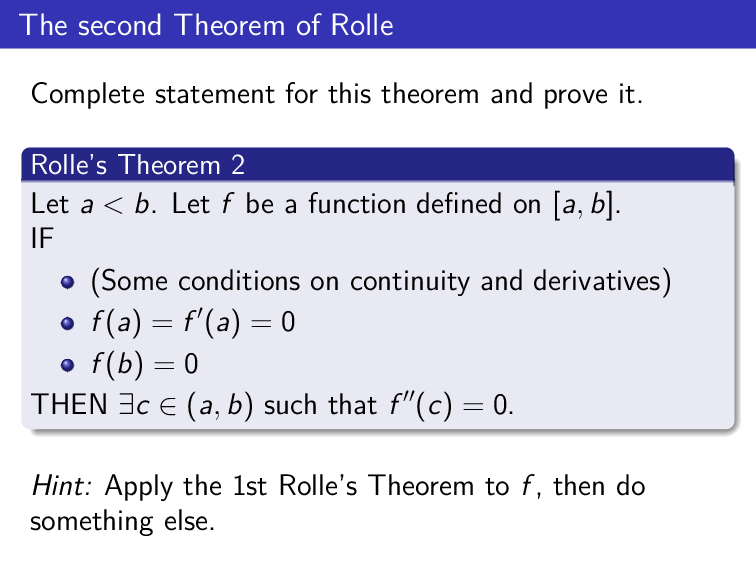
The second Theorem of Rolle
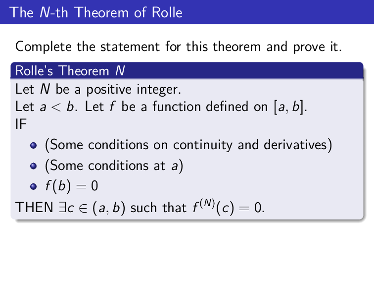
The $N$-th Theorem of Rolle
Warning. This is a great exercise to introduce students to the art of coming up with new theorems (as long as they are the ones exploring, rather than you telling them the answer), but it is harder and more subtle than it may seem. Do not underestimate it!
-
The point of this question is to introduce students to the art of coming up with new theorems (research?): explore, make conjectures, try to find the “minimal” hypotheses for a conclusion, focus on writing precise statements, and writing proofs.
It is not that this theorem is particularly important. (Well, in a way it is. This lemma simplifies a lot the proof of Lagrange theorem for the Remainder of a Taylor polynomial.)
-
This works well with just the first slide, or with both.
-
I like to tell them to just try to write the proof, and keep track of what hypotheses they are using about continuity and derivatives, and at the end write them up in the statement. This is, after all, the way research is done! But it is something weird for them, and they won’t be comfortable with it at first.
-
There is a big error or point of confusion. For Rolle’s Theorem 2, the proof goes like this:
-
Use Rolle’s Theorem on on .
-
This produces such that .
-
Use Rolle Theorem on on .
Therefore, the natural statement of the theorem will require the hypotheses:
-
is continuous on
-
exists and is continuous on
-
exists on
Of course, we could require stronger hypotheses, but it is a good exercise to think of the “minimal theorem”. Do not assume students will easily understand what I mean by this!
Students are likely to instead use a hypothesis like “ is continuous on ”, which would make the statement totally meaningless. Understanding why, and how to fix it, is pretty hard for them.
-
-
Like in most proofs in this unit, it is good to get students in the habit of verifying the hypotheses of a theorem before using it. They do not do it by default.
Related Videos
A new theorem
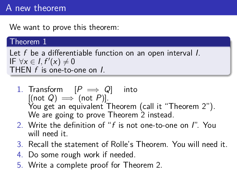
A new theorem
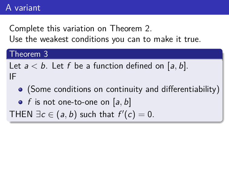
A variant
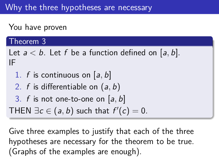
Why the three hypotheses are necessary
-
The point of this question is to introduce students to the art of coming up with new theorems (research?): explore, make conjectures, try to find the “minimal” hypotheses for a conclusion, focus on writing precise statements, and writing proofs.
It is not that this theorem is particularly important.
-
You can use all 3 slides, or stop at any point.
-
Slide 1 “A new theorem”:
-
We have not formally introduced “proof by contrapositive”. Rather, the hints lead students to discover proof by contrapositive, by understanding that the two “if-then” statements are equivalent. I much rather prefer that than a memorized algorithm.
-
Students will think that Theorem 1 is trivial. They think that the hypotheses implies the derivative is always positive or always negative, and thus the function is always increasing or always decreasing. However, since does not need to be continuous, this is not something we can assume.
-
-
Slide 2 “A variant”. (See the solution in Slide 3). The point is to understand the recurring theme in most results in Unit 5: it is enough to request continuity on the end-points, but differentiability everywhere else. Students won’t necessarily understand what “the weakest conditions possible” mean, or why we may want that.
-
Slide 3 “Why the 3 hypotheses are necessary” is self-explanatory. Doing this exercise is good practice whenever we learn a new theorems, but it is not something students would think of doing by default.
MVT - True or False?
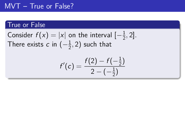
MVT — True or False?
-
Simple, warm-up question to check whether students have watched the videos. (The function is not differentiable on the interior of the interval.)
-
A recurring theme in this unit: before using a theorem, we need to verify its hypotheses.
Related Videos
Car race
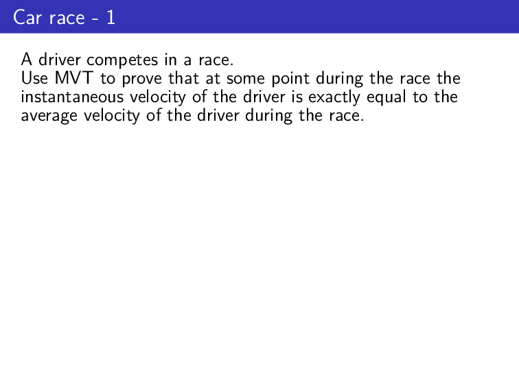
Car race - 1
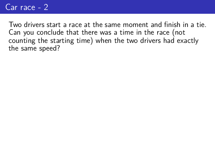
Car race - 2
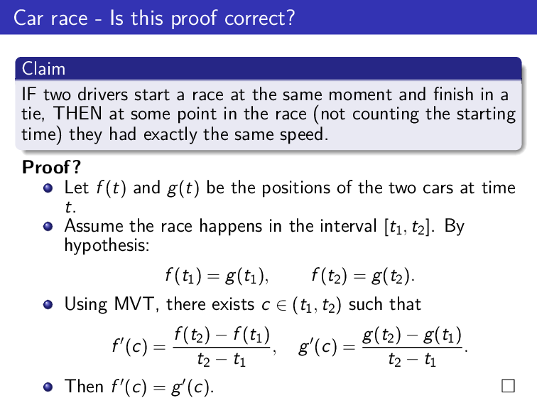
Car race - Is this proof correct?
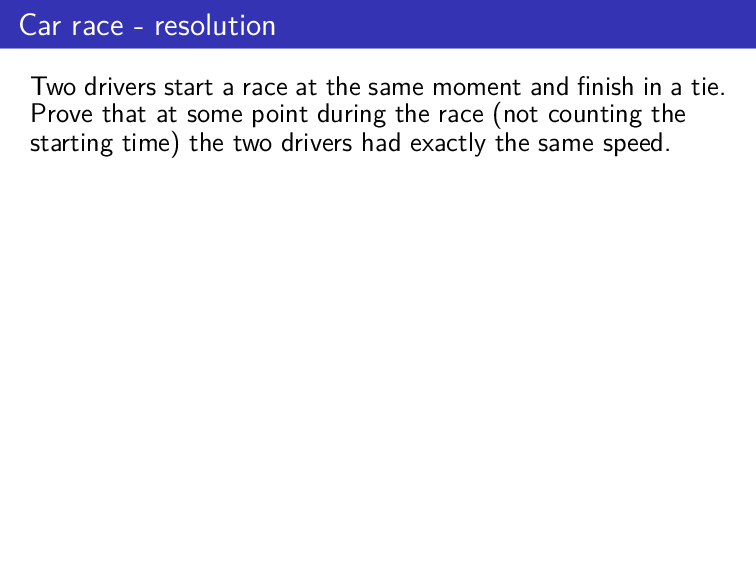
Car race - resolution
-
These slides play with the interpretation of the Mean Value Theorem. They start easy, and end up pretty tricky.
-
The Mean Value Theorem was introduced in Video 5.7, but the video is never explicit in the interpretation “the average rate of change of a function equals the instantaneous rate of change at some point”. Slide 1 (“Car race -1”) focus on this interpretation. I find this a necessary warm-up, or students will not know what to do.
-
The claim is true (even though the proof in the third slide is wrong). The key is to consider the function and apply MVT (or even Rolle’s Theorem) to it. This is not easy, and student will not think of this without help.
-
A possible plan to use these slides:
-
Use Slide 1 as a warm up. Only move on once students are happy with this interpretation.
-
Present the question in Slide 2. Invite students to think individually, then to discuss with their neighbours.
-
Then take a poll.
-
Some students may think the answer is yes because they are using the idea in the wrong proof in Slide 3. Using the slide if necessary, invite the students to find error by discussing with each other. Some students will find it, and once they explain it, it is convincing.
-
Alternatively, some students may think that we can only prove something weaker: that there are times (distinct for the two racers) when their speeds are the same. This is basically fixing the bad proof in the most straightforward way. It is worth it to acknowledge that this is a true result and invite a student to explain it.
-
-
Then surprise student with Slide 4 and tell them that the claim is still true! They will need a hint for it. We can tell them that since MVT only talks about a single function, we need to rewrite the condition “” into a condition about one single function. A strong student may get it with this hint, but most students won’t. Then, suggest they they use the function .
-
Related Videos
Speeding ticket
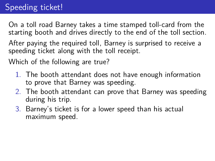
Speeding ticket!
-
If this question comes after the question “Car race” (or at least after the first part of that sequence), it is much easier.
-
Both 2 and 3 are true. To justify 3, we need to interpret the situation physically: at the starting and ending times Barney was not moving, so his speed cannot possibly have been constant.
Related Videos
Proving difficult identities
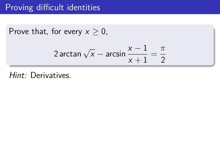
Proving difficult identities
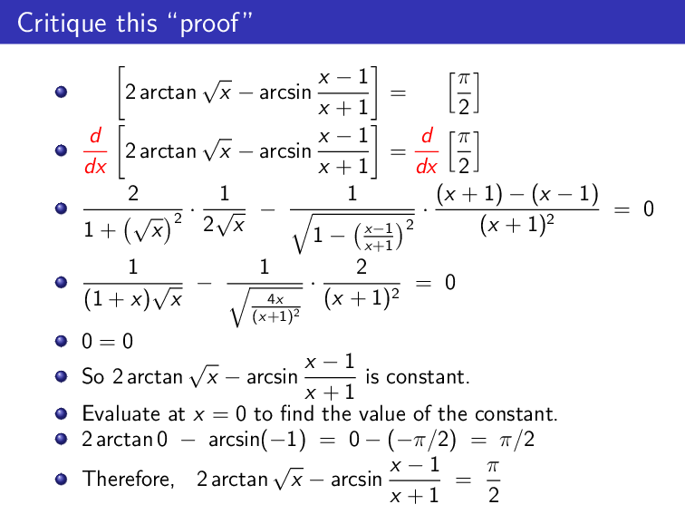
Critique this “proof”
-
There are two errors in the sample proof:
-
The proof write-up is bad. We should be defining a function, computing its derivative, realizing is 0, then concluding the function is constant. Rather, we are starting from the conclusion!
-
The function is not differentiable at 0! So we have only prove the identity for . We need to notice that is continuous at (on the right) to extend the identity to . Even when we point out the error, students are unlikely to say that the solution is to notice continuity.
-
-
For background, we have asked questions like this in past tests. The two errors in this proof are very common. In particular, a majority of the students make the second error. They are good at doing computations, but they do not like to stop and verify domains or check the hypotheses of the theorems they are using.
-
How I use this question:
-
I present the first slide and give students plenty of time (the computation is a bit long). They spend all their time focusing on computing and simplifying the derivative. They have not realized that there is anything else to do.
-
Once enough of them have gotten somewhere, I present the bad proof. I give them enough time to think about it individually.
-
I invite them to discuss with each other.
-
I take volunteers. Hopefully they will point out the errors. We can fix the first one, but we will probably be stuck on the second one.
-
If nobody has a solution for the second error, I point out what we have proven already (that the identity is true for all ) and I ask them to focus on how to prove that a function that is constant on must also be constant on . “What property must the function sastisfy?” It is still not easy, but it helps (some of) them figure it out.
-
I end with the moral: “Don’t do computations on autopilot. Every time you use a theorem, think about the hypotheses you need before you are allowed to use it.”
-
Positive derivative implies increasing
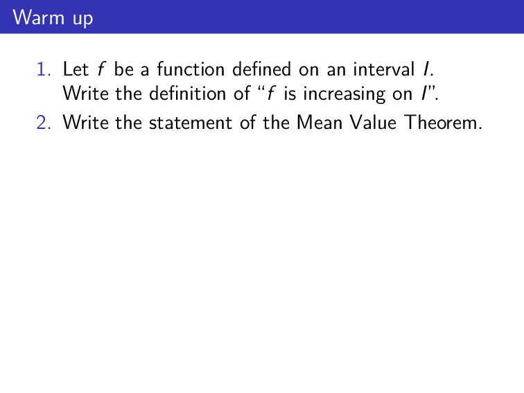
Warm up
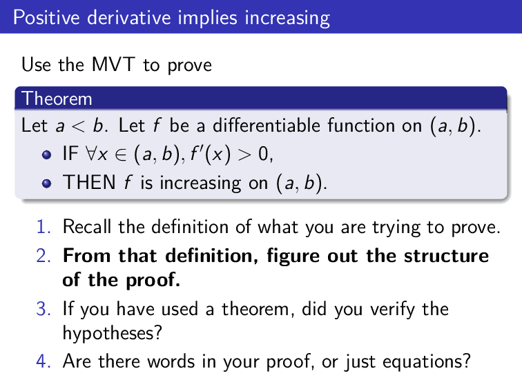
Positive derivative implies increasing
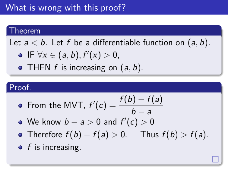
What is wrong with this proof?
Warning. This is possibly the most important activity in Unit 5. Do not skip it!
-
Coming up with a proof of this difficulty is one of the main objectives of the course. Don’t underestimate it: most student butcher it.
-
Video 5.9 contains the proof that “zero derivative implies constant” which is essentially the same. It is important that we give students the chance to write this proof themselves (rather than see us write it) and find the error themselves. If instead we simply write it ourselves, they will think they understand it and they will never realize they would have written it badly.
-
For background, in the past we have used this question in class; then we asked students for the equivalent proof for decreasing functions on a test. Half of them got it wrong. The bad proof you see in “What is wrong with this proof?” was more common than a good proof.
-
The warm-up slide is to ensure they actually write down those two things and they have them present when trying to write the proof. Otherwise they are careless.
-
The steps/hints/suggestions/checklist are supposed to help them clean up their proof. Specifically, writing out the definition of increasing and writing out the structure of the proof from it, before doing anything else, should make them realize the big problem with the bad proof.
-
How I use this question: I want them to do all the work. I won’t write the proof myself. If they need to see a sample proof, they can watch Video 5.9.
-
I give them Slide 1. I tell them to look the answers up if necessary but to write them down.
-
I give them Slide 2 without the four suggestions. I give them time to work individually. After a while, I show the suggestions and invite them to continue.
-
After a while I invite them to share proofs with each other and give each other feedback.
-
I shared Slide 3. I invite them to discuss the errors in the bad proof with each other.
-
I take volunteers to explain the errors.
-
Your first integration
Your first integration
- Many students will get the correct answer very quickly. However, they probably will just write down the calculations. They may not be able to explain what they are doing or what theorem they are implicitly using.
Related Videos
Intervals of monotonicity
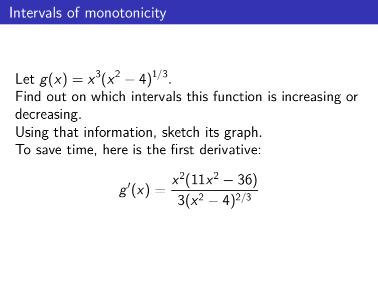
Intervals of monotonicity
-
Students do these questions pretty well. They probably already learned it in high school. Even if they didn’t, it is identical to the example in Video 5.12, and it is just following an algorithm.
-
The one issue that is likely to appear is whether the intervals of monotonicity include the endpoints. For example, is increasing on or on ? The answer is, of course, on both. Students are still confusing “increasing” with “positive derivative”. They sometimes even say “but is not increasing at ” and they need to be reminded that a function is increasing on an interval, not at a point.
Here we need to remind that the results from the videos say that “IF is any interval, is positive on the interior, and is continuous on , THEN is increasing on .”
True or False - Monotonicity and local extrema
True or False — Monotonicity and local extrema
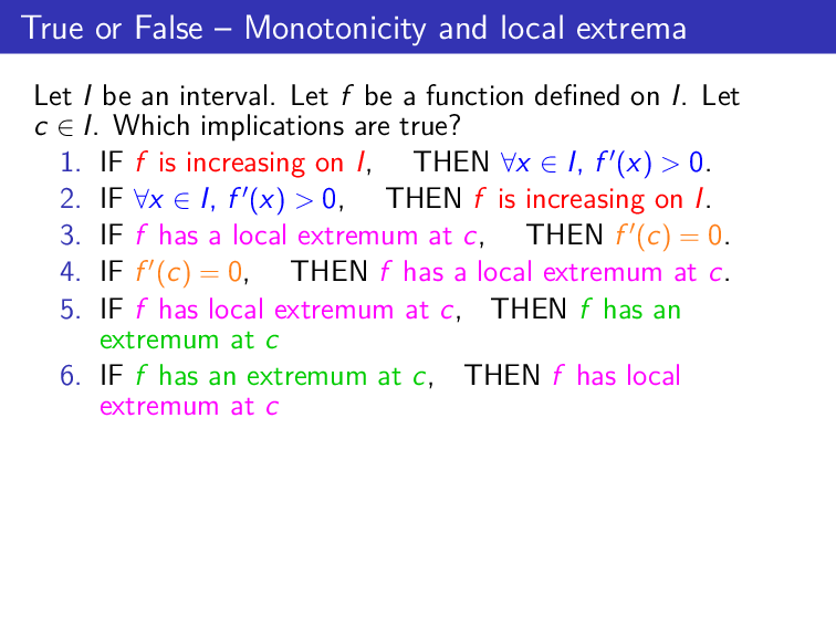
Warning. Don’t underestimate this question. It addresses a very common misunderstanding. I recommend not to skip it.
-
Many students will get this wrong. They may (mistakenly) think that
-
the definition of increasing is “positive derivative”.
-
“local extremum”, “critical point”, and “zero derivative” mean the same.
-
-
Only 2 is true.
-
1 is false: , .
-
3 and 4 are false. The correct statement is “IF has a local extremum at , THEN or DNE”. There is nothing else we can say.
-
5 is false, of course.
-
6 is also false according to our definition. An extremum at an end-point does not count as a local extremum. This is the standard criterion in single-variable calculus, but it is not the criterion in other courses.
-
Inequalities
Inequalities
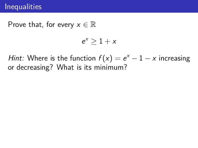
- This type of application has not been introduced in the videos. That is on purpose. I hope that the hint (plus discussion with each other) is enough for them to figure out how to solve this problem. Then I like to point this out: how they could figure out how to solve a problem that I had not taught them yet, and how this is one of the objectives of the course.
Backwards graphing
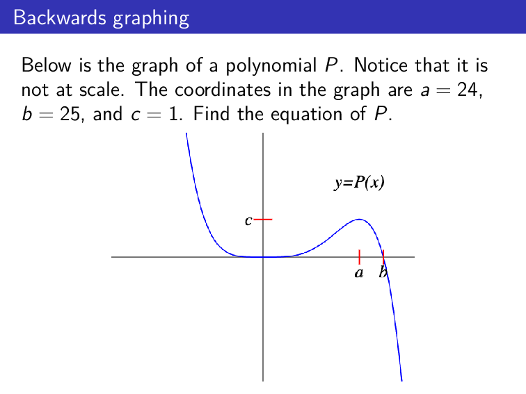
Backwards graphing
-
This question revisits the relation between the first derivative and monotonicity backwards. It will test whether students are comfortable with the concepts or only with using a fixed algorithm. It also requires some creativity. It is a great question, but hard to use effectively in class.
-
The first step is to conjecture that the polynomial probably looks something like
where is an even number and is a positive real. Once students realize this, they can do the rest. However, I do not have a great suggestion on how to guide students to discover this step without plain telling them.
A sneaky function
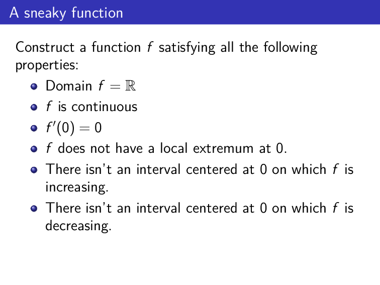
A sneaky function
-
This question is an interesting challenge, but it is hard to use effectively in class: most students will simply not know what to do and wait. If that is what happens, it is not worth it.
-
A possible solution is
Simple warm-up question to make sure students understand the definition of local extremum and (global) extremum.
There are normally two issues:
They miss the local maximum at x=4
They are not sure if x=6.5 (and other such points) counts as a local extremum, and they would like us to confirm it.
If I tell them to write down the definition of local maximum/minimum and redo the question, they are normally able to solve the question correctly. Then I remind that they should not do the problems by definition and not “by intuition”.